This post will outline the setup of Python application and its usage examples.
All necessary files can be found in the Wizzdev GitHub repository under fpga_data_transfer_demo/python/src.
To perform data acquisition a bitfile generated from corresponding VHDL sources is required.
How to setup Python environment.
We recommend creating a separate virtual environment for this project.
python3 -m venv venv
To activate the environment:
source venv/bin/activate
All required packages are listed in the requirements.txt file in the /python directory. All but one can be installed by calling :
pip install -r requirements.txt
while pyqtgraph must be installed from devel branch from its git repository as its latest release does not support Pyside2:
pip install git+https://github.com/pyqtgraph/pyqtgraph
Now GUI application can be started by calling:
python start_gui.py
assuming you are currently in fpga_data_transfer_demo/python/src directory, else just provide the full, or relative path to the start_gui.py script.
Using the application
The main functions of this Python application are:
- Online data acquisition – receiving data from FPGA and writing it to hdf5, with data real-time data visualization,
- Offline data viewer – hdf5 file reading and displaying saved data as time-series
At a start, the menu will show up. The parameters on the left side
Output directory is the directory where the resulting hdf5 file will be saved to,
Path to bitfile is the path to a previously generated FPGA configuration file,
Sources determine the number of sources that are generating the data,
Sampling rate is the sampling rate for each data source,
Packet length is the length of the whole packet (including ID and checksum) in bytes.
If the bitfile name follows this scheme:
4_1k_512B.bit
where: 4 is the number of sources, 10k is 10kHz sampling rate and 512B means 512-byte packet length (change them to values used for generics in your demo_top.vhd !), the application will automatically load these values to associated fields, otherwise they can be typed by hand.
It is important to provide the correct values, as wrong may cause errors in saved data or even disallow the data reception at all.
Online data acquisition
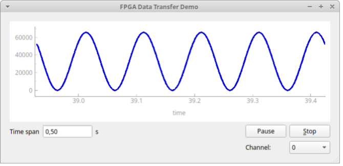
To start the data acquisition fill all the fields on the left side panel and press “Start”. Remember that the board must be connected and powered on. The bitfile will be uploaded to the board using the Opal Kelly FrontPanel library, and it usually takes a few seconds. After the board is successfully configured the plot will show up with live data on it. Currently observed channel can be changed by selecting one from the list on the bottom right. The displayed time span can be altered by editing the field below the plot.
Only the last received samples for specified time span ale displayed, hence after pausing you will be able to explore this region only (but you can still change between different channels). The data is still saved to file, even when plotting is paused. The whole received data can be inspected after the acquisition, by opening the resulting hdf5 file in the offline viewer. To stop receiving the data click the “Stop” button.
Offline data viewer
To read an already generated hdf5 file, insert its path into a specified field on the right side menu panel, and press “Open”. Once again the plot will show up, but this time without “Pause”/”Stop” buttons and no time span specification. Mouse buttons and scroll can be used to navigate through the plot. Below is an example – result of an about 10 minutes long acquisition session.
That’s all. I hope that you liked our demo application, and if you are thirsty for more insights – stay tuned! In the next post, we will explain in more details what is under the hood of this simple Python project.